Computational models

Satellite Orbits

Satellite state vectors are computed within the simulation for each simulation epoch and used to determine the pseudorange measurements as well as satellite visibility and depending parameters. Two options exist for state vector computation:

• orbit integration
• ephemeris-based computation

Using ephemeris-based computation the given perturbed Keplerian elements from the scenario are directly used to compute the satellite state. In the other case these Keplerian elements are used only for initialization of the orbit integration module which is a numerical integration of the satellite state based on gravitational forces.

The simulation of satellite orbits using orbit integration is useful to simulate satellite orbit errors as they would appear in reality due to the non-perfect representation of the perturbed orbit by using Keplerian elements as used within the navigation message.

Using orbit integration the satellite state vectors are propagated based on the gravitational forces of earth, sun and moon. While for the earth a gravity field model up to a certain (configurable) degree is used, sun and moon are modelled as point masses only, which is sufficient due to large distance to these bodies. The propagation is computed using numerical integration based on a Runge-Kutta scheme that is taken from ^[1].

Satellite Clock Noise - Allan Deviation

Based on the satellite clock model, the Allan Variance parameters differ. The appropriate values are given in the table below.

Allan Variance:

where

• WFM: white frequency modulation
• FFM: flicker frequency modulation
• RWFM: random walk frequency modulation

Clock Type	Description
Rubidium	h0: 1.0e-23 h1: 3.0e-27 h2: 4.0e-31
Cesium	h0: 1.0e-22 h1: 1.0e-27 h2: 2.0e-32
Hydrogen-maser	h0: 2.0e-24 h1: 7.2e-29 h2: 1.76e-34

Receiver Clock Noise - Allan Deviation

For the receiver's LO simulation, the Allan Variance is computed via the same model as for the satellite clock. Based on the chosen clock model, the Allan Variance parameters differ. The appropriate values are given in the table below.

Local Oscillator	Description
Crystal Oscillator (XO)	h0: 2.0e-19 h1: 7.0e-21 h2: 2.0e-20
Temperature Controlled Crystal Oscillator (TCXO)	h0: 1.0e-21 h1: 1.0e-20 h2: 2.0e-20
Oven Controlled Crystal Oscillator (OCXO)	h0: 8.0e-20 h1: 2.0e-21 h2: 4.0e-23

Receiver Path

Two models (Interpolation or Propagation) for the receiver path computation are provided. Depending on the settings, a certain model can be chosen.

In general, the following characteristics apply for both models:

• The earth-fixed receiver state (position, velocity, acceleration) is either set or computed for each simulation epoch.
• The receivers attitude and angular-velocity are computed for every epoch
• User defined input specifies the receiver states at certain relative timestamps (in order to be independent of changing simulation start and end times).
• If only one receiver state position is set (no velocity or acceleration), the receiver is treated as static.
• For interferer-based trajectories (Spoofer, Jammer, Spectrum-matched Jammers) attitude computation is not available.

State Interpolation

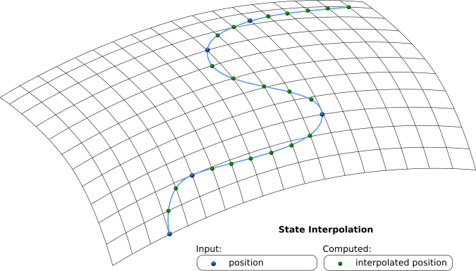
• When state interpolation is chosen, only the defined positions (nodes) are utilized (velocity and acceleration is neglected).
• The movement is simulated as geodetic lines (on the WGS84 ellipsoid) between these nodes. The geodetic line maintains its velocity after the last defined node.
• Interpolation:
  • The travelled distance is interpolated as a cubic spline interpolated function of time.
  • Additionally the cubic spline of travelled distance has to be monotone (rising) to ensure that the absolute velocity is never below zero.
  • Absolute velocity and acceleration are computed as derivatives of the travelled distance and applied to the unit vector of receiver direction at each point.
  • The receiver position is computed as first geodetic principle on the ellipsoid.

Note

The monotone cubic spline interpolation follows the algorithm published in ^[2] to ensure monotonicity (further information on the implementation can be found on Monotone Cubic Interpolation (opens new window))

First and Second Geodetic Principal

The computation of the receiver position is done as mentioned above using an interpolation on the ellipsoid for which solutions of the first and second geodetic principal on the ellipsoid are necessary. The first geodetic principal denotes the computation of the coordinates of a target point given the start point coordinates as well as direction and distance to the target point and the second geodetic principal is the reverse operation of computing direction and distance based on the two coordinate pairs. In Cartesian space these operations are quite trivial, however on the surface of an ellipsoid this is not true anymore. Since especially for longer distances there is a difference between the Cartesian and ellipsoidal solution the ellipsoidal formulae are implemented within the simulation. The principals on the ellipsoids are solved using the algorithm presented by Carl Friedrich Gauß^[3] with the extension that also the height above the ellipsoid can be different for start point and target point. The formulae for implementation are taken from ^[4].

State Propagation

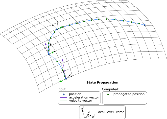
• When state propagation is chosen, the set position, velocity and acceleration are utilized.
• The position has to be provided as absolute WGS84 coordinates, whereas the velocity and acceleration are defined in a LLF (north, east, up).
• Every state is propagated via the previous state for every simulation epoch (an initial state is needed).
• Only one component (position, velocity, acceleration) has to be provided (the other two are optional).
• If a defined state is provided, it is directly applied for that epoch.

Note

• If only a velocity vector is provided, then the velocity vector is constant for the rest of the simulation. The position vector changes based on the velocity for every epoch.
• If only an acceleration vector is provided, then the acceleration vector is constant for the rest of the simulation. The position vector and velocity vector change based on the acceleration for every epoch.

Propagation Model

Provided Component	Description

Receiver Attitude and Antennas

Receiver Attitude and Receiver States

The Receiver attitude is explicitly defined by the user. For every waypoint the user can define roll, pitch and yaw. This attitude is defined from the local-level frame (LLF) to the body-frame. The corresponding rotation matrix is .

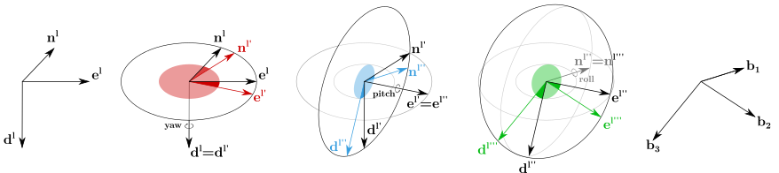
Rotation from Receiver LLF to body frame by yaw, pitch and roll angles

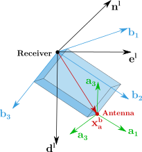
Receiver and antenna positions and their corresponding frames (LLF, body frame and antenna frame)

In agreement with the XPLORA concept, the user can select state propagation or state interpolation behavior of the trajectory simulation.

State propagation: The user defines the trajectory by means of receiver position , receiver velocity vector , receiver acceleration vector , attitude Euler angles (, , ) and angular velocity vector . Additionally an antenna position and an antenna attitude (, , ) can be defined for every antenna.

• Required state parameters for first state:
  • position
  • attitude
• After the first state, all parameters are optional
  • states: position, velocity & acceleration (optional)
  • attitude parameters: attitude & angular velocity (optional)

State interpolation: The user defines the trajectory by means of the receiver position and the attitude Euler angles (, , ). Additionally an antenna position and an antenna attitude (, , ) can be defined for every antenna.

• The velocity and acceleration are determined by the receiver positions given at certain points in time. The receiver position is interpolated between the defined positions (nodes) by using a cubic spline interpolation. The receiver velocity and acceleration is derived from the interpolated positions by the derivatives of the travelled distance.
• No has to be provided, since it is computed from two consecutives matrizes.
• Required state parameters:
  • position
  • attitude
  • all other parameters are ignored

Note

Attitude computation is only computed for Receivers, not for Interferers (Jammers, Spectrum-matched Jammers) or Spoofers.

Antenna position and attitude

A XPLORA receiver trajectory is the trajectory of the object, i.e. the state is the state of the origin of the body frame. If the position of the antenna is not identical with the BF origin, the lever arm (vector from the BF origin to the antenna phase center APC) will be used to compute the position, velocity and acceleration at the APC. The mounting position of an antenna is defined by means of its lever arm .

Moreover, if a relative rotation between AF and BF exists this has to be taken into account by definition of the antenna attitude. The antenna attitude is defined by a rotation from the BF to the AF.

• Antenna lever arm in the body frame:
• Antenna attitude: describes the antenna attitude with roll, pitch, yaw in the body frame. Rotates the body-frame (axes: , , ) to the antenna frame (axes: , , ).

Frame Definition

Description	Abbreviation	Vector & Matrix Sub/Superscript	RHS or LHS
Earth centered earth fixed frame	ECEF		RHS
Local level frame	LLF		RHS
Vehicel body frame	BF		RHS
Antenna frame	AF		RHS

where RHS is a right-hand system and LHS is a left-hand system. Vectors:

• : receiver position vector in the ECEF frame
• : receiver position vector in the local level frame
• : antenna position vector, defined in the body frame
• : transmitter position vector (can be satellite , jammer , spoofer )

The context between ECEF ellipsoidal coordinates () and LLF cartesian coordinates (north, east, down: ) is shown in the graphic below:

Details

Object Attitude

Attitude angles: roll, pitch, yaw. Internally this sets up the matrix , which rotates from local level frame (axes: ) to the body frame (axes: ) by rotating in the order yaw, pitch, roll.

Angular Velocity

The angular velocity relative to the inertial frame observed in the BF is written as: . The angular velocity vector is visualized below. It consists of three angular change rates around the body frame axis .

The angular velocity can be directly observed by an IMU located at the origin of the body frame.

Atmospheric Effects

Atmospheric effects are simulated in two ways: ionospheric delay and tropospheric delay including respective noise components (noise simulation can be activated and deactivated independently). Delays are computed based on the model selected within the scenario and follow the algorithms presented in:

Troposphere models

• Troposphere mapping functions for GPS and VLBI ^[5]
• Estimation of tropospheric delay for microwaves from surface weather data ^[6]
• GPT2w ^[7]
• Galileo Reference Model ^[8]
• Saastamoinen ^[9]

Ionosphere models

• Klobuchar ^[10]
• ESA Nequick G model ^[11]
• IONEX TEC maps ^[12]

Multipath

Within XPLORA, multipath effects are simulated by utilizing a land mobile satellite (LMS) model which characterises the time-varying transmission channel between a satellite and a mobile user terminal ^[13]. Basically, an impulse response model for wideband channels is implemented, which can be distinguished into three regions:

• Direct Path
• Near Echoes
• Far Echoes

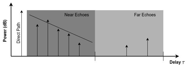
Note

Since Far Echoes are not relevant when modelling multipath effects based on GNSS signals, this region is neglected.

Direct Path Model

Within the Direct Path region, the probability function will differ from LOS conditions when shadowing is present. ^[14] For LOS conditions, a Rice distribution describes the probability density function (PDF) of the signal amplitude with

,

where the pre-determined Rice-factor denotes the carrier-to-multipath ratio corresponding to a specific environment. In shadowed environments, the PDF becomes a Rayleigh type with a lognormal-distributed mean power :

Near Echoes Model

For near echoes, the mean power is exponentially decreasing, where

,

with being a fixed delay and and representing the deterministic mean power loss and being pre-determined model parameters corresponding to a certain environment.

Following ^[14:1], the delay distribution follows an exponential distribution with

,

where the pre-determined parameter again corresponds to a certain environment.

Obstruction types within XPLORA

Within XPLORA, for every user (receiver), a multipath obstruction mask can be defined, with four possible obstruction types to be chosen from (for every azimuth and elevation angle pair) with a grid resolution of five degrees:

• LOS
• LOS+Echoes
• Echoes-only
• Obstructed

Environmental types and respective parameters

^[13:1] defines five types of depicting environments and provides a set of parameters for each model (direct path and near echoes) at certain elevation angles of the incoming signal:

• Open
• Rural
• Suburban
• Urban
• Highway

The environments' respective parameter sets are used within XPLORA. Refer to ^[13:2] for lookup tables providing the parameters.

Note

XPLORA parses the lookup table parameters from files. Therefore, the parameters can be easily adapted if needed.

Interference

An arbitrary number of interference signals can be added to the simulation for the simulation of unintentional RF interference or jamming signals using various customizeable waveforms. Each signal has its own transmission location and transmit power, which is used to compute the received signal power at each receiver based on a Friis free-space path-loss equation.

Spoofing

Multiple spoofers can be added to the simulation, which represent replicas of the respective satellite's authentic signal with a certain delay that is based on the location of spoofer and receiver as well as the simulated receiver position of the spoofer. Furthermore it is possible to add an additional code offset (in terms of pseudorange offset) to the spoofing signal to simulate imperfections of the spoofing signal alignment with the authentic ones.

Specular Point Computation

A simplistic model for computing reflected GNSS signals based on a specular point determined via a reference ellipsoid/surface is implemented. The specular point is obtained via a non-linear optimization, where a constrained cost function is used. In case the specular point shall be computed via a respective surface, a Digital Surface Model (DSM) is used.

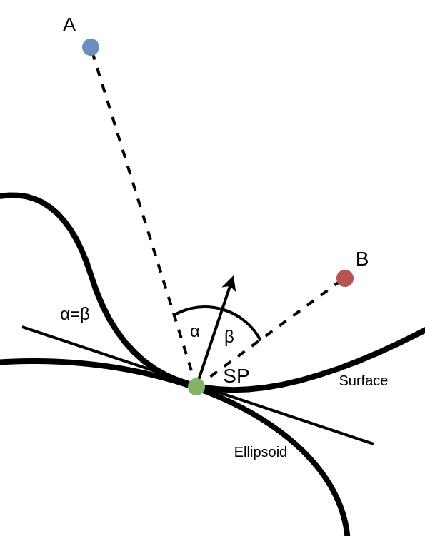
Non-linear optimization with ellipsoidal/surface projection as constraint

In the following, the algorithm for the specular point computation is described:

1. Define coordinates for both points (e.g. GNSS satellite) and (e.g. spaceborne receiver)
2. Compute initial specular point

3. Setup a non-linear optimizer with a constrained cost function (e.g. Nelder-Mead (opens new window) method) for minimization
4. Project the specular point on the ellipsoid/surface (constraint)
   • Ellipsoid
     with and being the semi-major and semi-minor axis of the reference ellipsoid
   • DSM

5. Compute the cost as the distance between , and :

6. Iterate until the cost or ingoing specular point coordinates are not significantly changing anymore
7. Computed the incident angle and reflection angle via the normal vector in and the unit vectors to point and
8. Check if and are the same
9. If not, redo minimization with different inital specular point (1.)

Note

All obtained DEM/DSM height values are transformed from orthometric to ellipsoidal height for the specular point computation.

---

1. O. Montenbruck and E. Gill, Satellite Orbits. Springer, Wien, NewYork, 2001. ↩︎

2. F. N. Fritsch and R. E. Carlson, "Monotone Piecewise Cubic Interpolation" SIAM J. Numer. Anal., vol. 17, no. 2, pp. 238–246, Apr. 1980. ↩︎

3. C. F. Gauß, "Untersuchungen über Gegenstände der Höheren Geodäsie" in Ostwald’s Klassiker der exakten Wissenschaften, 177th ed., J. Frischauf, Ed.Leipzig: Wilhelm Engelmann, 1910. ↩︎

4. B. Hofmann-Wellenhof and G. Kienast, "Bezugssysteme", Graz University of Technology, Graz, 2006. ↩︎

5. J. Boehm, B. Werl, and H. Schuh, "Troposphere mapping functions for GPS and very long baseline interferometry from European Centre for Medium-Range Weather Forecasts operational analysis data" J. Geophys. Res. Solid Earth, vol. 111, no. B2, p. n/a-n/a, Feb. 2006. ↩︎

6. J. Askne and H. Nordius, "Estimation of tropospheric delay for microwaves from surface weather data" Radio Sci., vol. 22, no. 3, pp. 379–386, May 1987. ↩︎

7. K. Lagler, M. Schindelegger, J. Böhm, H. Krásná, and T. Nilsson, "GPT2: Empirical slant delay model for radio space geodetic techniques" Geophys. Res. Lett., vol. 40, no. 6, pp. 1069–1073, Mar. 2013. ↩︎

8. A. Martellucci, “Galileo reference troposphere model for the user receiver” ESA-APPNG-ReF/00621-AM v2, vol. 7, 2012. ↩︎

9. Saastamoinen, J. (1973). Contributions to the theory of atmospheric refraction. Bulletin Géodésique (1946-1975), 107(1), 13-34. ↩︎

10. Klobuchar, J., 1987. Ionospheric Time-Delay Algorithms for Single-Frequency GPS Users. IEEE Transactions on Aerospace and Electronic Systems (3), pp. 325-331. ↩︎

11. Ionospheric Correction Algorithm for Galileo Single Frequency Users, Issue 1.1, June 2015 [ESA Nequick G Model] ↩︎

12. S. Schaer, W. Gurtner, 2015. IONEX: The IONosphere Map EXchange Format Version 1.1. Astronomical Institute, University of Berne, Switzerland ↩︎

13. Jahn, A. (2001), Propagation considerations and fading countermeasures for mobile multimedia services. Int. J. Satell. Commun., 19: 223-250. https://doi.org/10.1002/sat.699 ↩︎ ↩︎ ↩︎

14. A. Jahn, H. Bischl and G. Heiss, "Channel characterisation for spread spectrum satellite communications," Proceedings of ISSSTA'95 International Symposium on Spread Spectrum Techniques and Applications, Mainz, Germany, 1996, pp. 1221-1226 vol.3, doi: 10.1109/ISSSTA.1996.563500. ↩︎ ↩︎