# General Remarks
# Carrier Frequencies
The following carrier frequencies are available in the simulation:
| Name | Frequency [MHz] |
|---|---|
| L1/E1 | 1575.42 |
| L2 | 1227.60 |
| L5/E5a | 1176.45 |
| E5b/B2 | 1207.14 |
| G1 | 1602.00 |
| G2 | 1246.00 |
| B1 | 1561.098 |
# Channels
The following channels are available in the simulation:
| Channel | GNSS | Carrier | Detail |
|---|---|---|---|
| GPS L1 C/A | GPS | L1 | Coarse/Acquisition |
| GPS L2 C | GPS | L2 | C-NAV moderate + long |
| GPS L5 I/Q | GPS | L5 | C-NAV data + pilot |
| Galileo E1 OS | Galileo | E1 = L1 | I/NAV data + pilot |
| Galileo E5a OS | Galileo | E5a = L5 | F/NAV data + pilot |
| Galileo E5b OS | Galileo | E5b | I/NAV data + pilot |
| SBAS L1 C/A | SBAS | L1 | Coarse/Acquisition, includes EGNOS, WAAS & MSAS |
| GLONASS G1 C/A | GLONASS | G1 | Coarse/Acquisition |
| GLONASS G2 C/A | GLONASS | G2 | Coarse/Acquisition |
| BeiDou B1 I | BeiDou | B1 | D1-NAV data |
| BeiDou B2 I | BeiDou | B2 = E5b | D1-NAV data |
| QZSS L1 C/A | QZSS | L1 | Coarse/Acquisition |
| QZSS L2 C | QZSS | L2 | C-NAV moderate + long |
| QZSS L5 I/Q | QZSS | L5 | C-NAV data + pilot |
| NavIC L5 SPS | NavIC | L5 | proprietary message |
# GNSS Signal Specifications
The following table gives an overview of the specifications of all supported GNSS signals:
| GNSS | Band | Code | Modulation | Code Length | Data Rate | Min. Sampling |
|---|---|---|---|---|---|---|
| GPS | L1 | C/A | BPSK | 1.023 | 50 bps | 2.046 MHz |
| P | BPSK | 10.230 | 50 bps | 20.460 MHz | ||
| L2 | P | BPSK | 10.230 | 50 bps | 20.460 MHz | |
| C | BPSK | 1.023 | 25 bps / 50 sps | 2.046 MHz | ||
| L5 | I/Q | BPSK | 10.230 | 50 bps / 100 sps | 20.460 MHz | |
| Galileo | E1 | OS | BOC | 1.023, 1.023 | 125 bps / 250 sps | 4.092 MHz |
| PRS-like | BOC | 15.345, 2.5575 | 125 bps / 250 sps | 35.805 MHz | ||
| E5a | OS | AltBOC (E5) | 15.345, 10.230 | 25 bps / 50 sps | 20.460 MHz | |
| E5b | OS | AltBOC (E5) | 15.345, 10.230 | 125 bps / 250 sps | 20.460 MHz | |
| E5 (E5a+E5b) | OS | AltBOC | 15.345, 10.230 | - | 51.15 MHz | |
| E6 | PRS-like | BOC | 10.230, 5.115 | 125 bps / 250 sps | 30.69 MHz | |
| SBAS | L1 | C/A | BPSK | 1,023 | 250 bps / 500 sps | 2.046 MHz |
| GLONASS | G1 | C/A | BPSK | 0.511 | 50 bps / 100 sps | 1.023 MHz |
| G2 | C/A | BPSK | 0.511 | 50 bps / 100 sps | 1.023 MHz | |
| QZSS | L1 | C/A | BPSK | 1,023 | 50 bps | 2.046 MHz |
| SAIF | BPSK | 1,023 | 250 bps / 500 sps | 2.046 MHz | ||
| L2 | C | BPSK | 1,023 | 25 bps / 50 sps | 2.046 MHz | |
| L5 | I/Q | BPSK | 10,230 | 50 bps / 100 sps | 20.460 MHz | |
| E6 | LEX | BPSK | 5,115 | 2 kbps / 250 sps | 10.230 MHz | |
| BeiDou | B1 | I | BPSK | 2,046 | 50 bps / 50 sps | 4.092 MHz |
| B2 | I | BPSK | 2,046 | 50 bps / 50 sps | 4.092 MHz | |
| NavIC | L5 | SPS | BPSK | 10,230 | 50 bps | 20.460 MHz |
| S | SPS | BPSK | 10,230 | 50 bps | 20.460 MHz |
# Trajectory Map and Routing
# Import a route
To import a route, one has to perform the following steps:
- Right click in the map and choose a starting point for the route and a destination (Figure a).
- Possible routes between the points are shown in grey (Figure b).
- Choose one of the routes which are shown by clicking on them. Once a route is selected, the route is colored in blue and the route import icon
 becomes available (Figure c).
 - Click the import icon to import a new route to the trajectory model.
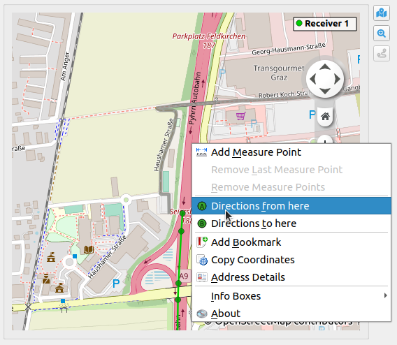 (a) Choose starting point and destination.
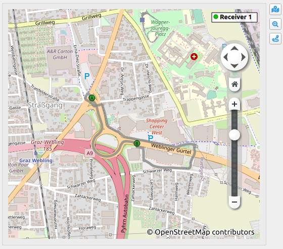 (b) Possible routes are shown in grey.
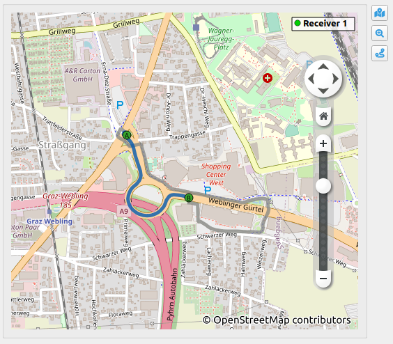 (c) One of two available routes were chosen.
- The import route dialog is shown, which shows the start and end point of the route, the total distance covered, the number of waypoints and each waypoint in a table view. The user can select the average velocity with which the distance is covered.
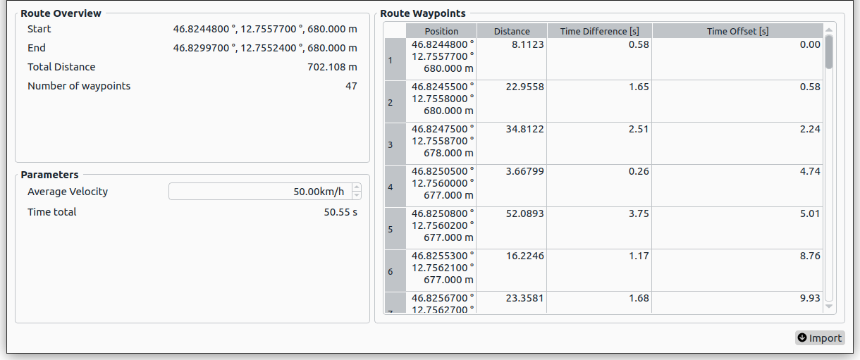 The import route dialog.
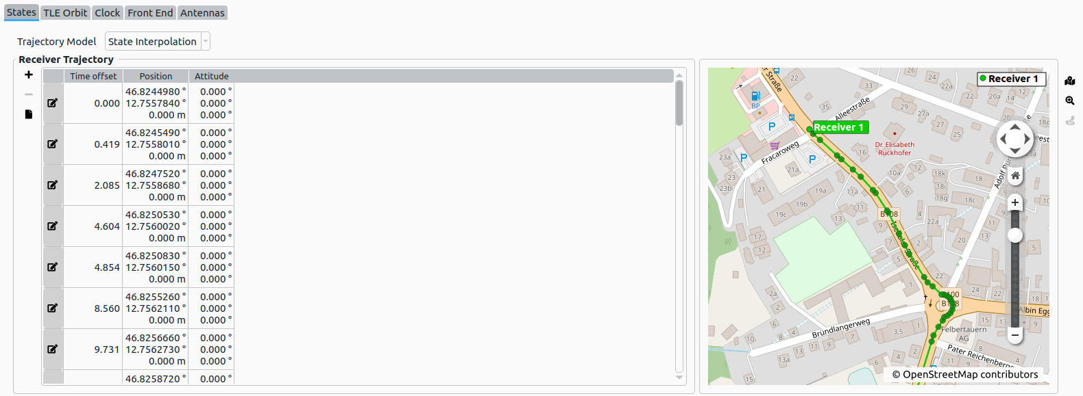
- Once the import dialog is accepted, the route waypoints are loaded into the trajectory table.
The route was successfully imported to the trajectory model.
# Trajectory Definition
Note
Trajectories can be defined for:
- Receiver
- Jammer
- Spoofer
- Spoofer Position
- Simulated Receiver Position
- Target Position
- Spectrum-matched Jammer
- Spectrum-matched Jammer Position
- Target Position
A description of the computational receiver path model can be found in the section Receiver Path. The receiver path is set by sequential way-points defined by:
| Parameter | Available in Propagation / Interpolation mode | Description | Remarks |
|---|---|---|---|
| Time offset | Propagation and Interpolation | A time offset (in seconds) from the scenario start epoch | |
| Position | Propagation and Interpolation | Ellipsoidal coordinates in WGS84 reference frame (Latitude [°], Longitude [°], Height [m]) | |
| Velocity | Propagation only | A velocity state vector is defined in the local-level frame with the position as it's origin and the following components:
| |
| Acceleration | Propagation only | A acceleration state vector is defined in the local-level frame with the position as it's origin and the following components:
| |
| Attitude | Propagation and Interpolation | - | For receiver simulation only |
| Angular Velocity | Propagation only | - | For receiver simulation only |
- A static receiver is defined by a single position with a time offset of 0 seconds and both of velocity and acceleration vector set to 0.
- A receiver trajectory can be defined by adding/removing single way-points using the
 or
or  buttons left of the table.
 - A receiver trajectory can be edited by using the
 button within the table.
NOTE
The attitude computation is only available for receiver trajectories. Interferer Attitude (Jammers, Spectrum-matched Jammers, Spoofers) is not simulated.
- The receiver path is computed via a defined model. The user can choose between two models (see Receiver Path Model for details).
- Interpolation
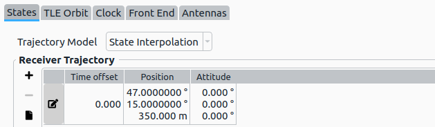
- Propagation
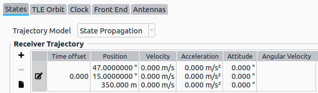
- Interpolation
NOTE
As long as the values in the tables are blank, values of the previous epoch will be set for all consecutive epochs.
For example:
- Epoch 1:
- Velocity [10.0 m/s, 0.0 m/s, 0.0 m/s] sets the velocity for all consecutive epochs to [10.0 m/s, 0.0 m/s, 0.0 m/s], if they are left blank.
- As soon as a new velocity is set for an epoch, that new velocity is set for all consecutive epochs.
- For details on receiver attitude computation see Receiver Attitude and Antennas
The trajectory can also be imported from a file  . Currently NMEA or KML files are supported to import way-points.
- The NMEA file must contain valid GPGGA messages. All other NMEA message types are currently not considered. The data from the file will replace all existing way-points.
- The KML file must contain
<Placemark>tags accompanied with a<TimeStamp>record. For more information on the KML format see KML File Format.
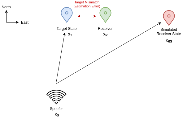
# Spoofing Trajectory definition
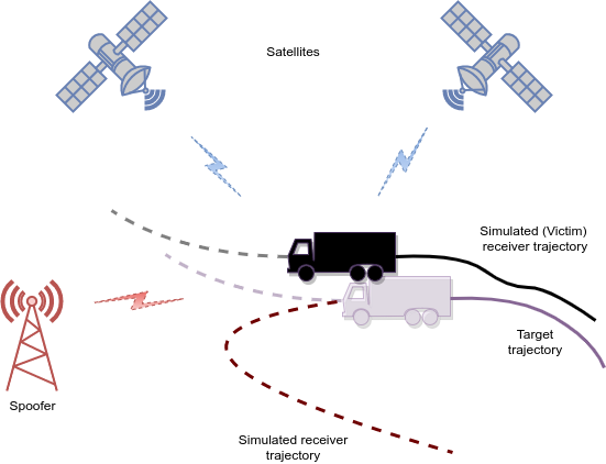
In order to cover several possible spoofing options, three different trajectories concerning spoofing have to be defined.
Position Types
| Position Type | Description |
|---|---|
| Spoofer position | The position of the spoofer, defined as state. |
| Simulated Receiver Position | Receiver position as simulated by the spoofer. |
| Target Position | Estimation of the receiver position done by the spoofer. |
Note
In order to perform optimized spoofing, the target position should be defined exactly as the receiver position of the receiver to be spoofed. This ensures, that correlation peaks of the spoofed signals overlap with the authentic satellite signals received by the receiver.
On the other hand, if an authentic spoofing scenario is required, then the attacker is probably unaware of the exact victim (receiver) position, thus the definition of the target position is provided.
Details
The defined target position is a way to simulate imperfect synchronized spoofing scenarios, in that the attacker does not know the exact victim receiver position. The difference between the real receiver position and the target position is called target mismatch
# Spectrum-matched Jammer definition
# Signal
The authentic GNSS signal can be written as:
where
The spectrum-matched jammer transmits a signal
# Trajectory
The spectrum-matched jammer trajectory is defined by two positions, the jammer position and the target position.
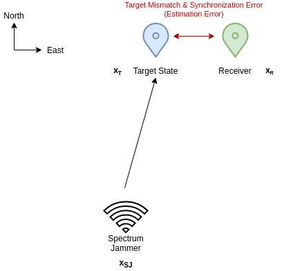
| Position Type | Description |
|---|---|
| Receiver Position | The real receiver position, defined as state. Configured in the Receiver tab. |
| Spectrum-matched Jammer position | The position of the jammer, defined as state. |
| Target Position | Estimation of the receiver position done by the jammer |
Details
The defined target position is a way to simulate imperfectly synchronized spectrum-matched jammer scenarios, in which the attacker does not know the exact victim receiver position. The error is called synchronization error and consists of two components:
- Target Mismatch
- Synchronization Error standard deviation
The total synchronization error
The synchronization error